Contents
Ejercicio 1
Imprimir una tabla formateada (entero y real) del logaritmo natural de los números 10, 20, 40, 60, y 80. Sugerencia: usar el comando fprintf y vectores
x=[10;20;40;60;80];
y=[x,log(x)];
fprintf('\n numero natural log\n')
fprintf('%4i \t %8.3f\n',y')
 numero natural log
  10 	    2.303
  20 	    2.996
  40 	    3.689
  60 	    4.094
  80 	    4.382
ejercicio2
%Hallar el vector X para la siguiente ecuación matricial:
A=[4 -2 -10;2 10 -12;-4 -6 16];
b=[-10 32 -16]';
x=A\b
x1=inv(A)*b
x =

    2.0000
    4.0000
    1.0000


x1 =

     2
     4
     1
Ejercicio3
Para la matriz de coeficientes anterior hallar la factorización LU, es decir A = LU y aplicar a continuación X = U-1L-1B para resolver el sistema anterior.
[L U]=lu(A)
x1=inv(U)*inv(L)*b
L =

    1.0000         0         0
    0.5000    1.0000         0
   -1.0000   -0.7273    1.0000


U =

    4.0000   -2.0000  -10.0000
         0   11.0000   -7.0000
         0         0    0.9091


x1 =

     2
     4
     1
Ejercicio 4
%Hallar  los autovalores y autovectores de la matriz A:
A=[0 1 -1;-6 -11 6;-6 -11 5];
[X,D]=eig(A);
fprintf('\n Autovectores (Columnas de la matriz)\n')
X(:,1)
fprintf('\n Autovalores (Diagonal)\n')
 Autovectores (Columnas de la matriz)

ans =

    0.7071
    0.0000
    0.7071


 Autovalores (Diagonal)
Ejercicio 5
%calcular los voltajes de los nodods y la potencia de la fuente
Y=[1.5-2j -.35+1.2j;-.35+1.2j 0.9-1.6j];
I=[30+40j;20+15j]
V=Y\I
S=V.*conj(I)
I =

  30.0000 +40.0000i
  20.0000 +15.0000i


V =

   3.5902 +35.0928i
   6.0155 +36.2212i


S =

   1.0e+03 *

   1.5114 + 0.9092i
   0.6636 + 0.6342i
Ejercicio 6
function TorresHanoi(n, i, a, f) if (n > 0) TorresHanoi(n-1, i, f, a); fprintf('mover disco %d de %c a %c\n', n, i, f); TorresHanoi(n-1, a, i, f);
end
TorresHanoi(5,'a','b','c')
mover disco 1 de a a c
mover disco 2 de a a b
mover disco 1 de c a b
mover disco 3 de a a c
mover disco 1 de b a a
mover disco 2 de b a c
mover disco 1 de a a c
mover disco 4 de a a b
mover disco 1 de c a b
mover disco 2 de c a a
mover disco 1 de b a a
mover disco 3 de c a b
mover disco 1 de a a c
mover disco 2 de a a b
mover disco 1 de c a b
mover disco 5 de a a c
mover disco 1 de b a a
mover disco 2 de b a c
mover disco 1 de a a c
mover disco 3 de b a a
mover disco 1 de c a b
mover disco 2 de c a a
mover disco 1 de b a a
mover disco 4 de b a c
mover disco 1 de a a c
mover disco 2 de a a b
mover disco 1 de c a b
mover disco 3 de a a c
mover disco 1 de b a a
mover disco 2 de b a c
mover disco 1 de a a c
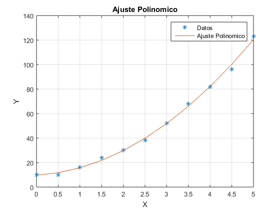
Ejercicio 7
%ajuste de polinomio
x=0:0.5:5;
y=[10 10 16 24 30 38 52 68 82 96 123];
p=polyfit(x,y,2)
yc=polyval(p,x)
plot(x,y,'*',x,yc)
xlabel('X'),ylabel('Y'),grid,title('Ajuste Polinomico')
legend('Datos','Ajuste Polinomico',2)
p =

    4.0233    2.0107    9.6783


yc =

  Columns 1 through 7

    9.6783   11.6895   15.7124   21.7469   29.7930   39.8508   51.9203

  Columns 8 through 11

   66.0014   82.0942  100.1986  120.3147
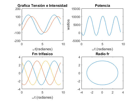
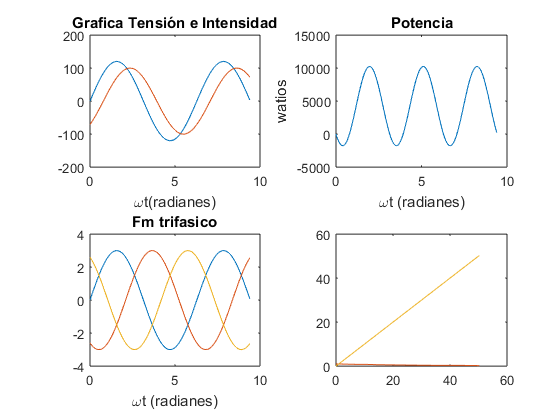
Ejercicio8
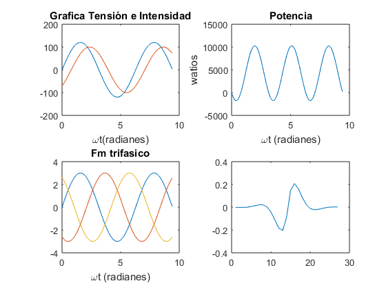
omegat=0:0.05:3*pi;
v=120*sin(omegat);
i=100*sin(omegat-(pi/4));
subplot(2,2,1)
plot(omegat,v,omegat,i)
title('Grafica Tensión e Intensidad'),xlabel('\omegat(radianes)')

p=v.*i;
subplot(2,2,2)
plot(omegat,p)
title('Potencia'),xlabel('\omegat (radianes)'),ylabel('watios')
Fm=3.0;
fa=Fm*sin(omegat);
fb=Fm*sin(omegat-2*pi/3);
fc=Fm*sin(omegat-4*pi/3);
subplot(2,2,3)
plot(omegat,fa,omegat,fb,omegat,fc)
title('Fm trifasico'),xlabel('\omegat (radianes)')

subplot(2,2,4)
fr=3.0;
plot(-fr*cos(omegat),fr*sin(omegat))
title('Radio fr')
Ejercicio 9
t=linspace(0,16*pi,100)
x=exp(-0.03.*t);
y=exp(-0.03.*t);
z=t;
plot(t,x,t,y,t,z)
t =

  Columns 1 through 7

         0    0.5077    1.0155    1.5232    2.0309    2.5387    3.0464

  Columns 8 through 14

    3.5541    4.0619    4.5696    5.0773    5.5851    6.0928    6.6005

  Columns 15 through 21

    7.1083    7.6160    8.1237    8.6314    9.1392    9.6469   10.1546

  Columns 22 through 28

   10.6624   11.1701   11.6778   12.1856   12.6933   13.2010   13.7088

  Columns 29 through 35

   14.2165   14.7242   15.2320   15.7397   16.2474   16.7552   17.2629

  Columns 36 through 42

   17.7706   18.2784   18.7861   19.2938   19.8016   20.3093   20.8170

  Columns 43 through 49

   21.3248   21.8325   22.3402   22.8479   23.3557   23.8634   24.3711

  Columns 50 through 56

   24.8789   25.3866   25.8943   26.4021   26.9098   27.4175   27.9253

  Columns 57 through 63

   28.4330   28.9407   29.4485   29.9562   30.4639   30.9717   31.4794

  Columns 64 through 70

   31.9871   32.4949   33.0026   33.5103   34.0181   34.5258   35.0335

  Columns 71 through 77

   35.5413   36.0490   36.5567   37.0644   37.5722   38.0799   38.5876

  Columns 78 through 84

   39.0954   39.6031   40.1108   40.6186   41.1263   41.6340   42.1418

  Columns 85 through 91

   42.6495   43.1572   43.6650   44.1727   44.6804   45.1882   45.6959

  Columns 92 through 98

   46.2036   46.7114   47.2191   47.7268   48.2346   48.7423   49.2500

  Columns 99 through 100

   49.7578   50.2655
Ejercicio 10
x=-4:0.3:4;
y=-4:0.3:4;
z=sin(x).*cos(y).*exp(-(x.^2+y.^2).^0.5);
plot(z)
Ejercicio 11
%hallar las raices del polinomio
p=[1 0 -35 50 24];
r=roots(p)
r =

   -6.4910
    4.8706
    2.0000
   -0.3796
Ejercicio 12
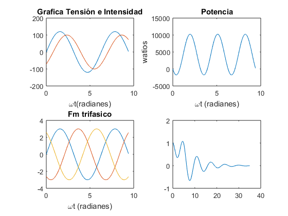
%function y = HalfSine(t, y, z)
%h = sin(pi*t/5).*(t<=5);
%y = [y(2); -2*z*y(2)-y(1)+h];

[t, yy] = ode45(@HalfSine, [0 35], [1 0], [ ], 0.15);
plot(t, yy(:,1))
Ejercicio 13
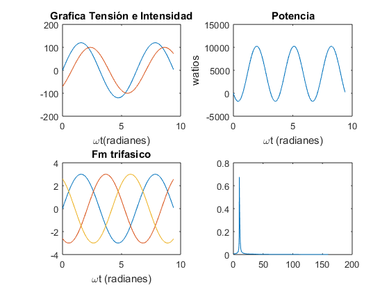
k = 5; m = 10; fo = 10;Bo = 2.5; N = 2^m; T = 2^k/fo;
ts = (0:N-1)*T/N; df = (0:N/2-1)/T;

g1 = Bo*sin(2*pi*fo*ts)+Bo/2*sin(2*pi*fo*2*ts);
An1 = abs(fft(g1, N))/N;
plot(df, 2*An1(1:N/2))

g2 = exp(-2*ts).*sin(2*pi*fo*ts);
An2 = abs(fft(g2, N))/N;
plot(df, 2*An2(1:N/2))

g3 = sin(2*pi*fo*ts+5*sin(2*pi*(fo/10)*ts));
An3 = abs(fft(g3, N))/N;
plot(df, 2*An3(1:N/2))

g4 = sin(2*pi*fo*ts-5*exp(-2*ts));
An4 = abs(fft(g4, N))/N;
plot(df, 2*An4(1:N/2))
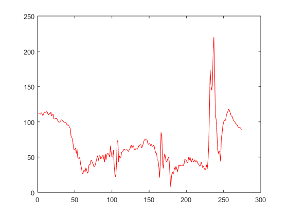
Ejercicio 14
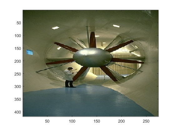
subplot(1,1,1)
A = imread('WindTunnel.jpg');
image(A)
hold on
figure
r= A(200, :, 1);
plot(r, 'r')
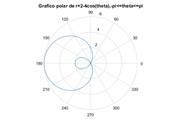
Ejercicio 15
theta = linspace(-pi, pi, 180);
r=2-4*cos(theta);

polar(theta,r)

title('Grafico polar de r=2-4cos(theta),-pi<=theta<=pi')